Part 3: Insurance companies performance based on price/book ratio in 2024
Insnurance companies
According to some guy from Columbia…
In my final article on this series of whether companies in certain sectors can be bought based on price to book ratio, I examine insurance companies. Recall that my original thesis is that, according to some well known financier whose name I forget, banks have assets that are impossible to value, and insurance companies have both assets and liabilities that are impossible to value. Even so, it is conceivable that any errors in valuation could be in the owner’s favor as easily as to their detriment. More to the point, the assets of these companies tend to consist largely of financial investments rather than, say, industrial equipment, so their book value tends to be a more reliable guide to their actual value and often times may be quoted regularly in the market. And so the naive strategy of evaluating these companies solely on their book value might be effective.
As we have seen, the correlation coefficient between a bank’s price/book ratio and its performance in 2024 was practically nonexistent, but when using tangible book value there was slight evidence of low price to book ratios producing outperformance when outliers are eliminated but at least in 2024 higher than average price to book ratios were not punished and even showed a tendency to be rewarded, which came as a surprise.
Turning now to insurance companies, the first complication is which book value to use. Insurance companies, particularly life insurance companies, make actuarial assumptions about life expectancy, interest rates, expected return on investments, and so forth. These assumptions are subject to change, of course, and as they change the value of the company’s liabilities change with them, sometimes dramatically, even though the company’s assets and near term cash flows are unchanged and a future shift in actuarial assumptions could erase the effect of the current ones instantly. The effects of these changes in actuarial assumptions are subsumed in “Accumulated Other Comprehensive Income” on the balance sheet, as these changes are not considered operating, since an insurance company is in the business of selling insurance and investing assets, not actuarial services.
However, insurance companies are in the habit of reporting their book value under GAAP and their book value not counting this accumulated other comprehensive income. By an extraordinary coincidence, of the fifty or so insurance companies that formed my sample, every single one of them reported a higher book value with this adjustment. Apparently, not a single insurance company has ever had its actuarial assumptions move in its favor in the history of the American insurance business. (Or, more likely, if they have the company sneakily counted it as operating income to make themselves look better). At any rate, in my opinion accumulated other comprehensive income, or more accurately, accumulated other comprehensive losses, should be included in book value, as it represents an economic loss, even if unrealized as yet, and a constraint on the insurance company’s business activities. This is also the view of a noted professor at Columbia School of Business.
Also, some insurance companies have goodwill, and eliminating that to arrive at tangible book value is another possible adjustment .
That said, what are our results? The Value Line, from which I draw my samples, divides insurers into life insurers and property and casualty insurers, the latter being much more numerous. There are also reinsurers, but not many of them so it is difficult to draw conclusions from such a small set.
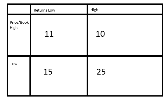
Among life insurers I was pleased to discover that in 2024 the naive strategy actually showed some signs of success, with a correlation coefficient of about 0.2 for both raw and tangible book value. Unsurprisingly, book value modified for accumulated other comprehensive income showed a weaker correlation. As I’ve said, given the numerous possible determinants of investment performance, one can hardly expect price to book ratio to be the sole factor in returns, but a correlation coefficient this high at least suggests that something is going on.
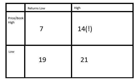
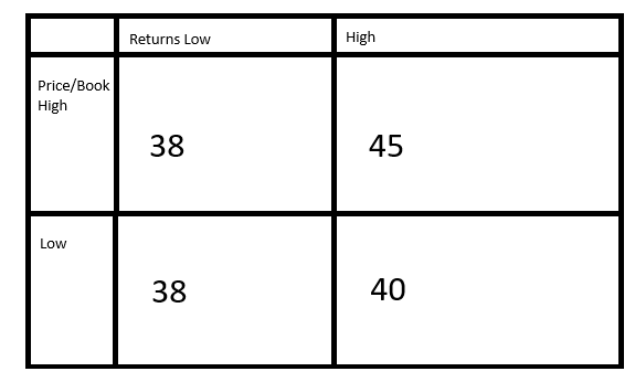
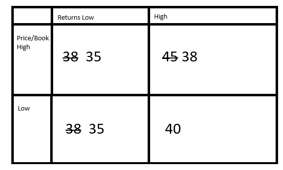
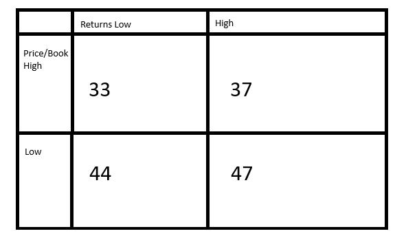
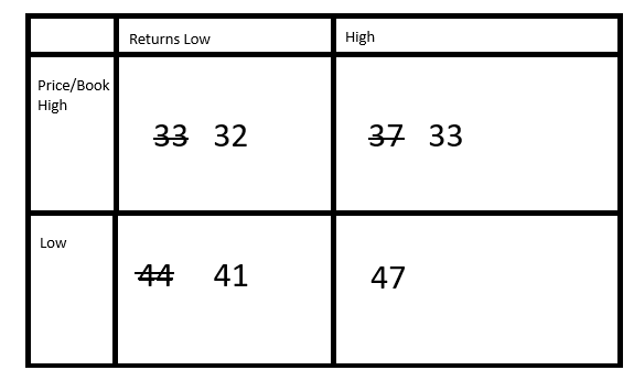
Among property and casualty insurers, I was disappointed to find a correlation coefficient of about 0.015, essentially consistent with no correlation. However, by dividing the outcomes into quadrants as before, I find that a higher than average price to book ratio was almost twice as likely to produce a lower than average return as a higher one, while a lower than average price to book ratio was more likely to produce a low return. Also, apparently 2024 was a difficult year for the average insurer, as returns were skewed to the downside.

So, to conclude, at least for 2024 the naive strategy of buying banks or insurance companies based on price/book ratio did not show reliable correlations apart from among life insurers. However, when purely considering if the price/book ratio was above average there were some minor indications of the validity of the strategy; with property and casualty insurers high price/book ratios were more likely to underperform, while with Midwestern banks, high price/book ratio banks showed above average returns but curiously that advantage disappeared when looking at tangible book values, to be replaced by a slight advantage for low price/book ratios, a sign that goodwill writeoffs are not overdue at least. And for non-Midwestern banks low price/book ratios had a slight advantage once outliers are removed, but curiously the high price/book outliers were more likely to outperform, which is counterintuitive and requiring further investigation. And of course this study should be extended to prior years.